„Bias in AI“ is a popular topic these days, and usually this just means that algorithms cannot be shamed into not picking up certain pattern in the real world.

Half a year ago OpenAI published the exploits of a new Deep Learning language model called GTP-2, without publishing the larger versions of the model itself. This language model can create text that is much more coherent than was previously possible. It is trained on 40GB of articles, which makes it likely that it is severely biased in the same way as our media seems to be.

The reasoning for not publishing the model was that its capabilities make it too dangerous to put into the wrong hands. It might for example make fake news much more convincing or easy to produce. But, now, several independent replications later they started publishing larger models with the latest one having almost half as many parameters as their largest one which is as of yet still unpublished.

As this is about the biggest model that would fit into my RAM anyway, I tested GTP-2’s grasp of HBD. The prompt is my text, the samples are created by the model, which aims to coherently build on the prompt. I only excluded one or two samples that didn’t turn out coherent or grammatical. For an overview I only cite the very first sentence after my prompt:

Model prompt >>> The persistent IQ and achievement gaps between different ethnic groups are predominantly due to …

Sample1:
… ipsilateral technical dominance, or their tendency to share innovative problems and productive parts, rather than being the result of genetics. Top performers in the tribal dress component are among the most genetically gifted officials both socially and economically.

Sample 2:
… condemns from lower socio-economic backgrounds , likely reflecting environmental factors or Aryans mining wealth in the Middle East ( Hu et al., 2002 ).

Sample 3:
… erythrocytosis deficiency which may be partially compensated by factors including cosmetic surgery.

Sample 4:
… differences in transactional culture.

Sample 5:
… under- or over-selection with strong negative and positive selection processes, respectively.

Sample 6:
… differences in immigration policy patterns.

Sample 7:
… ersatz”personal”classes, not to ethnic differences in cultural relatedness, a group standpoint evolutionary economist].

Sample 8:
… vernacular, cultural and cognitive factors.

Sample 9:
… prevalent racism and the subsequent exacerbated IQ gap has a high cost.

Sample 10:
… genetically determined differences in IQ with no other neutral or intergroup effects.

Sample 11:
… bias against European-descended Black Americans

Sample 12:
… vernacular education system, not to individual differences, says Alan Kendry, professor of social policy at Victoria University in Sydney.

Sample 13:
… vernacular media and behavioural aberrations derived from biased educational models.

I am not sure what’s up with „vernacular“ but you have to be impressed by the variety of responses. These results are not nearly as biased as I assumed, though of course still heavily shifted towards environmental explanations. Out of these 13 samples at least three give a genetic reason. The „selection“ answer continues „On the other hand, other studies (for example Eurogenes 2013 and Mandarin 2007) show a genetic basis for larger and more ancillary effects on test scores at the end of high school.“ and the „vernacular, cultural and cognitive factors.“ continues with „Untreated dysfunctions of some genes not only may contribute to the variation observed between and across ethnic groups, but may position racial and ethnic groups at disadvantage relative to other ethnic groups; for example, attenuating the manifest motor skills of Jews“

Let’s finish this post with some gems that stood out among the continuations of the above responses:

There has been a larger increase in IQ among the general public by a range of thousands points on the standardised IQ test across India ( Singh and Sharma, 1980 ; Das, 2001 ). Meanwhile, socioeconomic status is negatively related to ‘intelligence levels among youth of all economic groups in the country’ ( Bhatnagar et al., 2007 ).

Yeah, thousands of points, sounds about right.

No ethnic group raises future generations in the spirit of Western society and values, and different part of the ethnic group must adjust to what it must learn from the outsider, so different ethnicities can explain themselves why they were colonized, what conditions existed for Dalits to support the government in their ancestral homes and how to impose values on all Hindu Dalits.

A glimpse into a Hindu nationalist’s mind.

If everything else is equal, the Asian (though improving) male population is asked to step up and do STEM/STEM education; the Latino female population is asked to head start an obstetrics practice.

If only these male Asians would step up and do STEM …

Equally, I would like to add credit to try to clarify what (other than Jungian/Marxist Othering) science education is meant to teach. It is morally wrong to pursue “biological determinism” and “one of many evolutionary processes” to “conform to one’s moral outlook” and then exaggerate through social engineering to “profit by social engineering” and “make money by social engineering” in the process, and that is what mentioned below. …(incoherent blathering)… Our philosophy is the same as George Orwell’s Gestapo; still gags anyone who loses to us (our ideas are so evil!)

GTP-2 simulating a Marxist, only with unusual self-knowledge.

In the US all kinds of statistics are meticulously recorded on the basis of race or ethnicity. This kind of data is a luxury not easily afforded in many European countries, where we have endless debates about whether some ethnic group or other might be more prone to violent crime. In the US it is well known that African-Americans are roughly three-fold overrepresented in violent crime. This means that in US cities, the rate of violent crime is mostly determined by the percentage of the black population.

So in the US, instead, the debate can, though equally fruitlessly, cover the topic of possible causes and what best to do about them. One of these causes, eagerly championed by Steve Sailer, is the so called Ferguson effect. In the aftermath of black-lives-matter protests, crime rates allegedly spike, because the police walks back on discriminating but effective measure like racial profiling in frisk-and-stop.

Together with the Jussie Smollet case, this lead me to wonder whether black governance had an effect on black crime. If your key voters would punish you for the most effective measures against black crime, maybe you wouldn’t be so eager to implement these. Or maybe for a black mayor crime in the black community is a bigger priority and insights into how to alleviate the problem are more common?

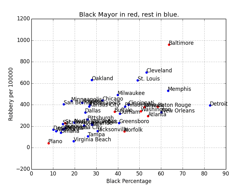
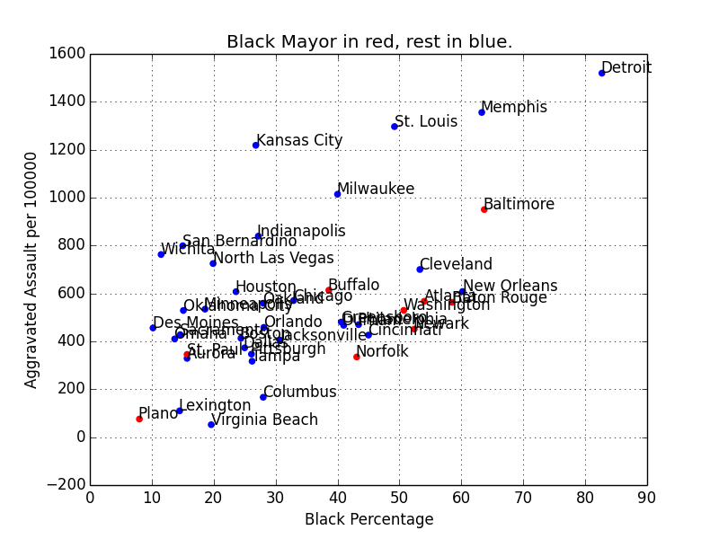
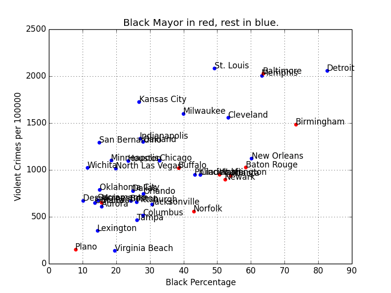
So I created a list of cities with their general and specific violent crime rates, as well as their black percentage [1] and cross-bred it with a list of black mayors [2]. Then I plotted black percentage against crime with every red dot a city with a black mayor and every blue dot a city without a black mayor. I am not sure how accurate and up to date these data is. And I am sure this analysis could be done in a much more principled way, but as a first look into the topic this gives already gives a clear tendency.

The correlation of black percentage and rape is much less tight than the other correlations. Would be interesting whether this is real or a result of more unreported cases.

Overall we see that cities with black mayor have less violent crime than other cities with the same black percentage. This trend is observable for all types of crime. And though there is a lot to be desired in our methodology, it seems unlikely that a more thorough investigation would yield the opposite result.

[1] Crime rate by city
https://en.wikipedia.org/wiki/List_of_United_States_cities_by_crime_rate

[2] Black mayors
https://blackdemographics.com/culture/black-politics/black-mayors/

[3] Black percentage
https://en.wikipedia.org/wiki/List_of_U.S._cities_with_large_African-American_populations

In the last blogpost we saw that the GDP-IQ relationship in multiethnic societies is probably roughly the weighted sum of the GDP predicted by the mean IQs of all ethnic groups. This indicates that low IQ immigration retards economic growth in a predictable fashion.

I don’t analyze this question to assign blame or even to make policy proposals, but simply to predict the future. It is a fact that in many Western countries the relatively high IQ native population is slowly being replaced by immigrants that on the whole don’t show the same cognitive performance (as measured for example by IQ-tests, PISA or other scholastic tests [1]).

In developed countries, economic growth generally isn’t very high. If the relative growth of the lower performing section of the population manages to significantly retard or even completely stall economic growth, we are in for a bad time.

In our first simulation we will compare the per capita economic output of a country, where the native population has a fertility rate of 1.4 and the missing kids are replaced by immigrants that show a 10 point IQ gap compared to the natives. This is roughly the situation of Germany and both in birth rate and IQ gap relatively extreme.

We use only the population between 20 and 65 for the calculation of GDP, the working age population. We also assume a simplified scenario, where suddenly the birthrate drops from replacement rate to 1.4 and the missing working age people are replaced by a homogenous immigrant group to hold the population exactly steady. Also all mothers are exactly 30 years old.

These artificial assumptions lead to a slightly bumpy ride. We see that the first twenty years nothing happens, because the missing kids aren’t working age yet. Then further thirty years down the road the decline speeds up, because the next generation of of mothers is now already coming from a low fertility generation. Then we hit the point where immigrants start leaving the workforce …

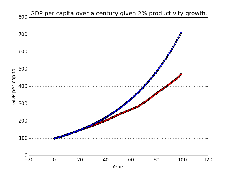
But the overall picture of a more detailed simulation wouldn’t be very different. Over 80 years the GDP drops to 66% of what it would be with a completely native population. Of course in reality this happens against the backdrop of economic growth stemming from productivity growth through innovation.

In developed countries the annual growth rate seems to hover around 2% [2]. This should already include immigration effects, but we can use it as a conservative estimate of possible future growth. In the second figure we see how the effect of low IQ immigrants making up an increasing share of the population plays out against a backdrop of 2% growth.

Fortunately, even these relatively extreme settings with low fertility and a big IQ gap do not seem to threaten to stall the economy completely. This makes sense because a 34% decline over 80 years corresponds to a shrinking of half a percent per year, which can still be set off by a normal rate of growth.

[1] IQ gap via PISA
https://akarlin.com/2012/05/berlin-gets-bad-news-from-pisa/
[2] Euro zone economic growth
https://tradingeconomics.com/euro-area/gdp-growth-annual

When I was analyzing the IQ-GDP connection [1], one of the big questions that I never quite got around to tackling, was how much the growing percentage of immigrant populations with lower mean IQ in western countries is expected to retard growth.

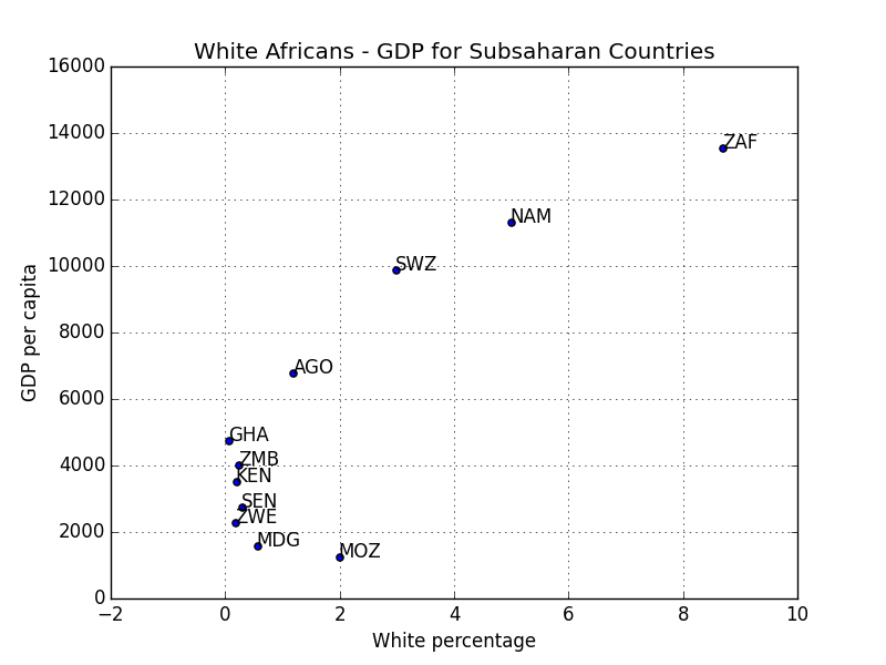
Of course that is not immediately a given. It is conceivable that low IQ immigrants to high IQ countries free up smart people for more complex jobs, so that the average productivity doesn’t take a hit. However, in my blogpost IQ-GDP: Ethnicity [2] we analyzed White Africans and Chinese Minorities in South-East-Asia and saw that the relationship between population percentage and GDP is extremely linear. This does not point towards strong non-linear effects. In all likelihood the GDP of a mixed population is roughly the same as the sum of the GDPs predicted by the IQ of the separate ethnic groups.

By the way, this also indicates that the mean IQ becomes unreliable as an economic predictor if the different ethnic groups have very divergent IQs. Namibia and South Africa for example punch way above their average IQ, because of their white minority. This is consistent with purely linear effects, because the exponential relationship between IQ and GDP will mean that the white minority affects the GDP much more than the average IQ.

The question is an important one, because growth is our way to run away from many social ills. It’s when the pie stops getting bigger that the fighting starts in earnest.

Unfortunately it is quite difficult to get accurate data on all the necessary variables. Essentially we are interested in the immigrant fraction of the working age population over time. But not just recent immigrants, but ideally a total breakdown of ethnicities and the size of the mixed population, plus accurate IQ-values. Good luck with that.

Instead I plan on doing a series of simulations, where we calculate how the IQ hit depends on the IQ gap and the fertility rate in Western Countries. We will assume that immigration is used to keep the population size roughly constant, i.e. to replace the missing kids and we will contrast the results with what we would expect if the birth rates had instead been kept at replacement level.

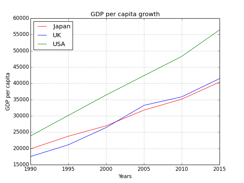
For now let’s contrast GDP per capita [4] and, what better captures the capability of an economy, GDP per capita of the working age population.

Here we see that the Japanese economy starting out with a clear advantage was decisively overtaken by the UK in the 2000s.

However, after controlling for the working age population [3] the story changes. Suddenly growth over the entire 25 years is very similar and Japan regains a slight lead after the 2000s. In our simulation we are going to focus on the working age population by calculating the changing makeup of each cohort.

[1] IQ-GDP
https://halfassed.science.blog/2019/02/23/iq-gdp-ii-curve-fitting

[2] IQ_GDP: Ethnicity
https://halfassed.science.blog/2019/03/10/iq-gdp-iv-ethnicity

[3] Demographics of the working age population:
https://en.wikipedia.org/wiki/Demography_of_the_United_Kingdom
https://en.wikipedia.org/wiki/Demographics_of_Japan#Aging_of_Japan
https://en.wikipedia.org/wiki/Demography_of_the_United_States#Percent_distribution_of_the_total_population_by_age:_1900_to_2015

[4] GDP by year and country
https://en.wikipedia.org/wiki/List_of_countries_by_past_and_projected_GDP_(PPP)_per_capita#IMF_estimates_between_1990_and_1999

In the last post we discussed that labor market discrimination in a functioning market is quite unlikely. But call-back rates for identical applications differ consistently by race or ethnicity. Even if we allow for ability differences, this seems difficult to explain without discrimination. Of course, if 50% of all companies hire in a discriminatory fashion and the other 50% are completely fair, the end result will likely be very minimal differences in wages or unemployment after controlling for ability while call-back rates can be quite different. This might still be part of the story.

However, even if all companies hire exactly according to the expected job performance of the applicants, call-back rates of applicants of different ethnicity will still differ even with an identical resume. The main reason for this is regression to different means. The qualification of an applicant can be seen as one measurement of his ability. His actual job performance can be seen as another. These two measurements will correlate imperfectly. Therefore the second measurement is expected to regress to the population mean.

If the population mean is lower for one ethnic group than for another, the expected regression to the lower mean leads to a lower expected job performance and therefore fewer call-backs.

Yes, that means that for every level of ability a member of a lower performing group will be expected to perform worse than equally able people of a higher performing group. This sure sounds like discrimination, doesn’t it? If for every level of ability one group is underestimated compared to the other, obviously the whole group has to be underestimated, right?

Well, actually not. This is an instance of the famous Simpson’s paradox, where a statistic can be the case for all subgroups but still not hold for the whole group. The easiest way to see this, is to realize that it doesn’t actually matter to which group you belong, if you look at people x standard deviations out from their group’s mean. An Asian-American who is one standard deviation above the Asian-American mean in terms of his qualification, will still be expected to only be 0.5 standard deviations above the Asian-American mean in terms of job performance (if we assume a correlation of 0.5 between qualification and job performance). So an Asian-American who is one standard deviation above his group’s mean in actual ability will be underestimated to the same degree as an African-American who is one standard deviation above his group’s mean. So summed over the respective bell curves the underestimation that both groups suffer is exactly the same.

The second statistical phenomenon that might play a role is the fat tail. If you create a cutoff above which you would want to interview a candidate, the group of people above the cutoff from the higher performing group will on average be more capable than the group of people above the cutoff from a lower performing group. This is due to the fact that bell curves drop more quickly the farther out from the tail you are.

So to get the same average ability and maybe the same success rate of candidates you might want to use a higher cutoff for applicants from lower performing groups. I am not suggesting that HR knows this. I am just suggesting that if you average over enough companies the practices followed might be close to statistically optimal. Otherwise you get arbitrage opportunities and those tend to be found and exploited (and if they are, they vanish).

In the US, there are persistent income gaps between Whites and Blacks [1]. They are generally explained by historical and current discrimination. Similar gaps exist between other ethnic groups and in other countries and of course between men and women.

Readers of this blog know, that there are equally persistent gaps in some cognitive abilities or behavioral patterns that might easily explain big parts of these gaps.

But there are other reasons to be skeptical of tales of labor market discrimination. Discrimination on the labor market creates arbitrage opportunities. If 99% percent of business owners are not willing to pay Blacks as well as Whites for the same work done, the 1% willing to do so have the opportunity to scoop up great workers for little money. It’s just free money, and if labor costs are a significant part of business expense this kind of discrimination quickly becomes unaffordable.

Now, labor market discrimination of course is in principle possible. In the above example, having a racist (or sexist) majority of 99% is surely enough to leverage social sanctions against the 1% and to consistently pay some groups less for the same work. But as soon as social sanctions against non-racists are no longer plausible, labor market discrimination becomes equally implausible.

But wait a second, isn’t there the well publicized phenomenon that fields into which women went when they entered the workforce saw a drop in wages? [2]

Well, when the iron curtain fell and Poles went into the business of harvesting asparagus in the West, the wages in this beautiful and traditional endeavor also declined precipitously. This is called wage dumping and it is the opposite of labor market discrimination. Poles were just willing to do the job for less.

And of course the same is true for women. Women are willing to accept lower wages for jobs that are compatible with family formation. I.e. low stress, part time, no travel, close by kinda jobs. They got into these jobs by wage dumping.

But how do we explain different call-back rates for equal resumes? There is a large literature on the fact that resumes that only differ in the identifiable ethnicity can have quite different call-back rates when applying for the same job [3]. This is a very rich and mathematically interesting question, that touches on key concepts like Simpson’s paradox, the normal distribution and regression to the mean, which is one reason why it is never accurately portrayed in the media. We are going to close that gap in the next post.

[1] Black-White income gap
https://www.economist.com/united-states/2019/04/06/the-black-white-wealth-gap-is-unchanged-after-half-a-century

[2] Female wage dumping
https://academic.oup.com/sf/article-abstract/88/2/865/2235342

[3] Different call-back rates by ethnicity.
https://www2.econ.iastate.edu/classes/econ321/orazem/bertrand_emily.pdf

In the last post we have seen that women on average bring fewer Elo points to the table if they draw tournament chess games against men. Fewer than if they would play other women and fewer than men would require to draw against men.

One explanation for this would be that men are more inclined to make disfavorable draws against women. In this scenario men would willingly donate Elo points to women instead of pushing for a win. Maybe because they try to specifically show goodwill to female opponents, maybe because they just can’t muster the same aggression as against male players.

However, this statistically robust phenomenon could also be due to confounding. The most realistic confounder is age or speed of improvement. Young players improve quickly. Therefore they will generally be stronger than their rating implies. This of course results in the effect that they will on average be lower rated than their opponent in drawn games.

To make sure that we are not chasing a chimera we bin our Elo differences by age for both male and female players against male opposition. Then we can look for each age group separately whether women have „drawing privilege“ compared to males of the same age. This takes care of the improvement issue, in fact it probably overcorrects, because boys probably improve a little faster.

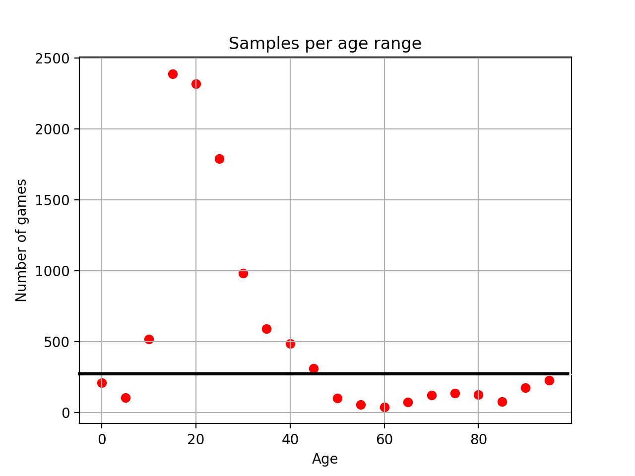
The following plot shows the number of games for each 5 year age span.

Here we have to confront an ugly truth: Our unique identification of players is not very unique. There aren’t actually any player of the age 0-5 and not many more at the age of 90+. These are noise, due to misidentification. However, the age groups 15-35 rise far above the noise, indicated in the figure by the black line, so this is the area where our results may be reasonably accurate. Additionally, we have to take the possibility into account, that the Elo difference in drawn games is an underestimate diluted by misidentified and possibly misgendered players.

Here are the corresponding Elo difference between male and female drawing players. Inside the black box are the observations where the sample number rose above the noise line in the earlier plot. The age groups 10-15 and 45-50 should maybe also be removed, but they fit the overall trend even if 10-15 is a major outlier.

So what do we observe? The female drawing privilege drops steadily with age. At age forty it is only half of what it used to be at age twenty. The effect size is slightly smaller, so maybe having many young players did make a difference. Overall we see that our results are not confounded by age. In fact they fit the theory very well that men are unwilling to try hard to beat young women.

Privilege is a hot topic currently. For some reason, one of the most obviously privileged demographic is rarely mentioned: Young women.

Young women have better educational outcomes. Earn more than their male counterparts in almost all bigger US cities. And are set to enjoy a significantly longer life.

On top of that, young women, especially if they are somewhat attractive, can count on support, leniency and favoritism from a significant number of men.

Of course many people would dispute that. A few years ago there was an interesting paper [1], showing that in chess men play more aggressive opening lines against female opponents.

The implication is that female chess players do not compete under the same conditions as male players do. An elevated aggressiveness could very well discourage women from competing in chess. A similar pattern could be present in the labor market as for instance at a job interview. If male recruiters treat female job applicants more aggressively than male applicants then women could be discouraged from applying for or accepting such jobs.

Patrik Gränsmark

The method used in this paper is quite crude and I hope to present a much more elegant way to determine risk taking and aggressiveness in chess in a later blogpost. But I do not doubt the result that men play more aggressive opening lines against women. However, I am less sure about the motivation behind this choice.

The authors of the paper seem to assume that the objective of this opening strategy is to beat the female opponent. They then show that the strategy backfires and men actually score slightly worse if they play more aggressively. But it could just as well be the case that men choose risky lines trying to impress their female opponents. In that case the choice would not be irrational despite the lower probability of winning. The optimal course of such a game might be a daring and creative gambit later followed by a generous draw offer.

These are two opposing interpretations of the same result. Either men go out of their way to beat women, or men are trying to impress the rare potential chess playing mate and don’t mind losing an Elo point or two on the way.

To get to the bottom of this puzzle we will analyze the draws, offered and accepted, between male and female players.

In chess, you can offer a draw after making a move, before you press the clock, and the opponent may accept the offer or make a move to continue the game. So in almost all cases the player to last make a move in a drawn game has been the player to offer the draw. If you want to keep your Elo at its current level, you are well advised to make draws against opponents that average the same Elo as you. But if you are favorably inclined towards a certain group, say young women, you might accept and make draw offers against players averaging a significantly lower Elo. Conversely, if you very much want to beat them, you might only accept draw offers by significantly stronger players.

We analyze two million chess games, trying to uniquely connect the players names to the fide player database. This allows us to determine sex, age and other interesting attributes. As we will see, it isn’t at all easy to uniquely identify the correct player and we only manage to do this for 30% of the players. Typos, varying initials and different transcriptions make this difficult.

Initially, I looked at games with both players above 1900 Elo and I distinguished between games longer than 20 moves or shorter, and between white offering the draw and black offering the draw, and between the women playing white and the man playing white.

However, I found that the result is always pretty much the same. In a drawn game between male players, or between female players only, black will be slightly higher rated (4 to 12 points). This makes sense, because it is compensation for the first move advantage that white enjoys.

If a male player makes a draw against a female player, compared to the baseline, the female player will be 40-50 points lower rated. So a women has to bring 40-50 fewer points to the table to make a draw (if playing a man).

Given that we sliced and diced the dataset into several parts, we can be sure that this result is very robust. Here are the values for the overall dataset, the first player is white, the number is the average Elo advantage of white:

Women against men: -62.7 points
Men against men: -10.0 points
Women against women: -8.8 points
Men against women: 43.96

Note the symmetry: It doesn’t matter who is white and who is black. The Elo loss for the men compared to the baseline of intra sex games is the same 52-54 points.

These numbers are based on more than 10,000 games between a man and a women and significantly more games by men against men.

This does not look like men are trying harder to beat women. In fact, it looks more like support, leniency and favoritism.

But it is not a slam dunk yet. In the following blogposts we will dig a little deeper, make sure we are not being confounded in any way and try to unveil the entire story.

[1] Men play more aggressively against women
https://en.chessbase.com/post/male-che-players-show-elevated-aggreivene-against-women
http://ftp.iza.org/dp4793.pdf

After looking at the rating gaps between ethnic groups, we will today turn our inquiring gaze towards the relative performance of women in chess. More than a decade ago, there was a paper that purported to explain the relative absence of female players at the very top by the low participation rate of women [1].

This never sounded particularly convincing to me, because if underrepresentation were the only reason, we would expect a women among the top twenty (at a 1:19 underrepresentation) and 5 women among the top 100. Instead there are 0 and 1 women in the top 20 and the top 100. I also knew that women average roughly 200 points lower in the German rating system. So a lower performance across the board based on differential ability or interest in the game seemed more likely.

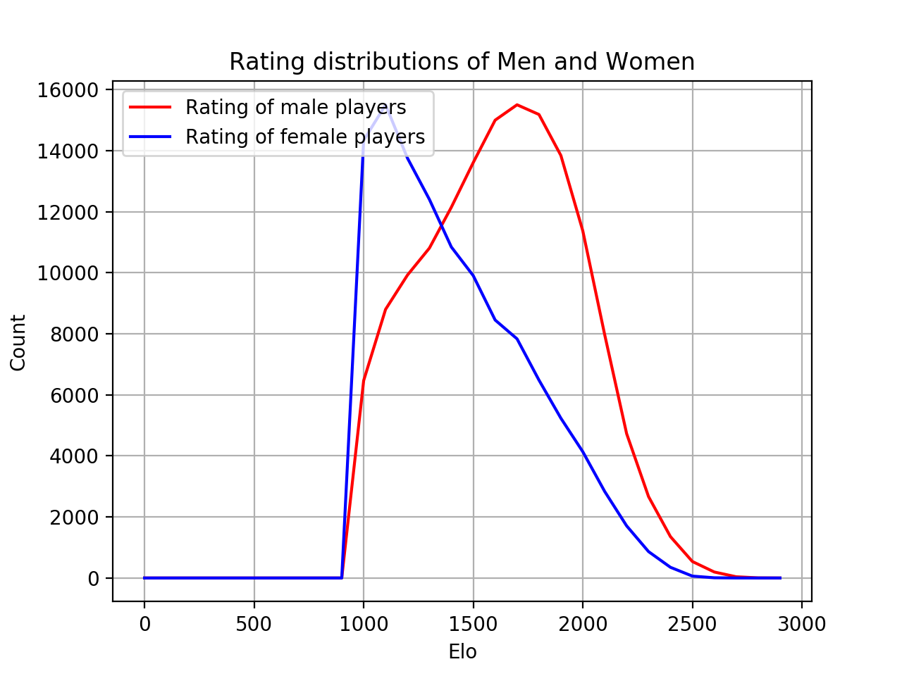
Initially, my investigation supported this suspicion. For 150,000 men and 16,000 women among the active chess players in my database, the men have on average roughly a 200 Elo advantage (1679 vs 1474). A closer look at the distributions, however, made it unlikely that this gap is due to innate differences.

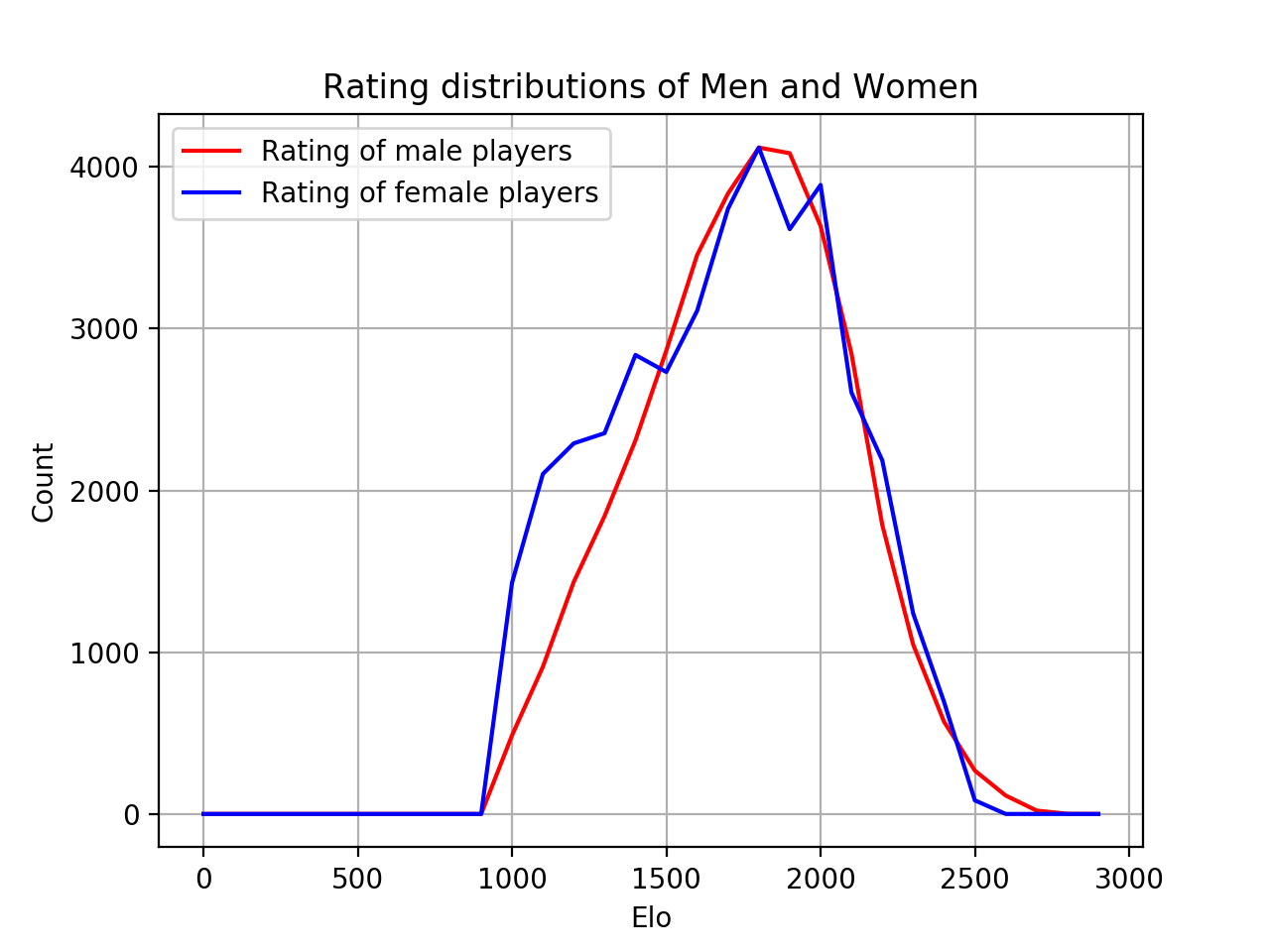
As we can see, the female curve is not even remotely gaussian. The true bell curve seems to be hidden under an avalanche of beginners. By restricting the dataset to those players born between 1960 and 1990, we eliminate most of the influence of age and almost all beginners.

Now, the avalanche of very weak players is almost completely purged and the bell curves become very similar. There is actually a female advantage between 2100 and 2400. Maybe this is the area where you are very good as a woman but nothing special as a man (the rating necessary for women titles fall into the space: 2100 for women fide master, 2200 for women international master and 2300 for women grandmaster).

After 2500 there is a distinct male advantage, which reproduces the observation that underrepresentation cannot explain the under representation at the very top. However, given that overall these bell curves are very similar and given that there was actually a women in the top ten only a decade ago, this doesn’t seem to point to innate ability differences.

Of course, underrepresentation can hide innate ability differences, if the female players are just sampled from a higher percentile of innate talent. But this is difficult to investigate and certainly beyond this blogpost.

[1] Why are the best women so good at chess?
https://www.researchgate.net/publication/23763925_Why_are_the_best_women_so_good_at_chess_Participation_rates_and_gender_differences_in_intellectual_domains

In the last post, we showed that US-American Ashkenazim have a higher average Elo rating than the average US chess player. In this post we extend the analysis to the ethnic and racial minorities African Americans, Asians and Hispanics.

Originally, I was just curious whether Asians had overtaken the Ashkenazim. This seems to be happening in several other measures of academic excellence. I assumed that to be the case, because chess rating first and foremost reflects how much work you have put into chess. So it likely responds strongly to the Asian work ethic.

When comparing Ashkenazim to the general US player I was methodologically quite lazy. I didn’t bother correcting for age because I assumed that the age structure would be similar enough. When looking at the Asian Elo this assumption no longer holds: Most current Asian chess players in the US are likely the kids of relatively recent immigrants.

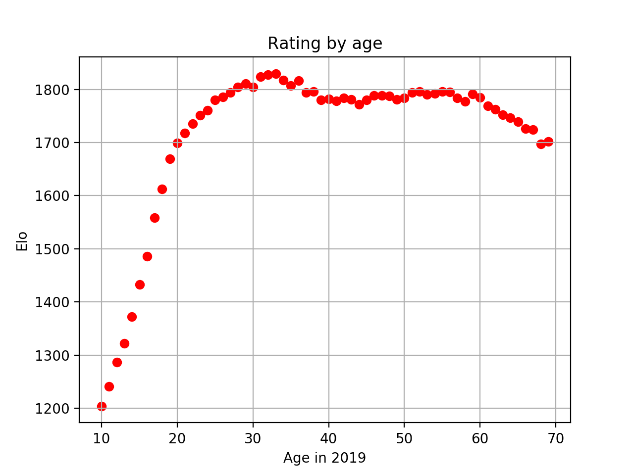
Indeed, the average birth year of Asian chess players in the US seems to be 2001 vs 1986 for all players. Instead of using Elo directly, we look at the deviation from the average global Elo for the given birth year. This allows us to eliminate the effect of age.

We use the 2010 US Census [1] to create samples of Asian, Black, Hispanic and White chess players. These are all players whose names belong with a >90% probability to the respective ethnic group. (For blacks we choose >80% probability, because otherwise the sample is almost nonexistent.) I restrict the samples to male players and birth years >1950.

I also create an additional Ashkenazi sample using my list of Ashkenazi names that occur among Israeli chess players and are not obviously mostly non-Ashkenazi (I excluded Perez, Miller, Brown).

This results in 420 Asians, 60 Hispanics, 66 Ashkenazim, 391 Whites, 14 Blacks. The low number of Whites and Blacks is a result of the difficulty of clearly distinguishing these two groups by surname. The high number of Asians is a result of uniquely Asian names. Ashkenazim are probably much more over represented than they are in my samples.

These are the age controlled deviations from the global average Elo for each group:
Asians 339
Ashkenazim 250
Whites 189
Hispanics 140
Blacks 125

With a White standard deviation of 215 we transform these numbers into IQ for a more intuitive comparison:

Asians 110.4
Ashkenazim 104.2
Whites 100.0
Hispanics 96.6
Blacks 95.5

The differences are probably distorted by weaker groups being more predominantly sampled from the right tail. But the ranking is quite unsurprising. After all, the 2019 US chess champions are called Hikaru Nakamura and Jennifer Yu [2]. With the much younger age structure US chess is bound to become much more Asian dominated in the future, with the ex-Soviets fading into the background.

[1] US census 2010
https://www.census.gov/programs-surveys/decennial-census/data.html

[2] US chess championship 2019
https://www.uschesschamps.com/2019-us-championships/2019-us-championship/overview